Pulse oximetry
Background
A pulse oximeter measures the oxygen saturation of the blood and changes in blood volume in a tissue by measuring the plethysmograph signal. The device is based on two physical principles: (1) the presence of a pulsatile signal generated by arterial blood; (2) the fact that oxyhemoglobin (O₂Hb) and deoxygenated hemoglobin (Hb) have different optical absorption spectra.
A pulse oximeter is usually clipped to an appendage, most commonly a finger, but sometimes an ear lobe or nose septum is used. A light source, usually an LED, on one side of the tissue penetrates through the tissue to be detected by a photodetector (usually a photodiode or a phototransistor) on the other side. As the light passes through the tissue, it is absorbed by various species. Much absorption happens in the tissue, some more in venous and capillary blood, and still more in non-pulsatile arterial blood. On top of all of that absorption is varying absorption due to pulsatile arterial blood. It is this varying absorption that is measured in pulse oximetry.
Pulse detection
The transmitted light intensity fluctuates from peaks to valleys according to the systolic and diastolic phases of the cardiac cycle. This fluctuation is typically measured in the IR region of the light spectrum, around 940 nm. The time-trace of this variation is directly proportional to the blood pulsatile motion. Therefore, we can use it to deduce the pulse rate, the number of beats per minute.
Measurement of oxygen saturation
In addition to measuring a pulse rate, we also wish to measure oxygen saturation, which is defined as the ratio of oxyhemoglobin to the total hemoglobin concentration. We cannot exactly measure this with pulse oximetry because we cannot take into account the contributions of nonfunctional hemoglobin, such as carboxyhemoglobin and methemoglobin. So, instead, we define the oxygen saturation, as determined by pulse oximetry, to be
To measure SpO₂, we consider absorption at a second wavelength in addition to the IR used to measure the pulse. Below, I show the absoprtion spectra for O₂Hb and Hb. Between about 600 and 800 nm, Hb has a higher extinction coefficient than O₂Hb. If we monitor transmission of light at this second wavelength, in addition to the 940 nM we are already using to detect the pulse, we can determine SpO₂. In particular, there is a big gap between the extinction coefficient of O₂Hb and Hb in the red region, around 660 nm, and the gap is the opposite as in the IR, where O₂Hb has a lower extinction coefficient.
Obtaining SpO₂ by monitoring transmission at 660 nm and 940 nm requires a bit of theory. To start, recall the Beer-Lambert Law.
where the left-hand-side is the ratio of the transmitted to incident light intensity, \(C\) is the concentration of absorbant species, and \(d\) is the path length. The extinction coefficient is dependent on the species and on the wavelength, as we can see in the spectra above.
The contributions of multiple absorbant species multiply (the product of the extinction coefficients and concentrations add). So in the case of light passing through a tissue, we have
where we have used the subscript “tissue” to denote all absorbing species besides those in arterial blood. Here, \(d\) is the path length through arterial blood.
During a pulse, the path length through the arterial blood increases due to dilation of the arteries. Let \(d_v\) be the path length through arterial blood at a “valley” of a pulse and \(d_p = d_v + \Delta d\) be the path length through arterial blood at a peak of a pulse. We can then write
where the v and p subscripts refer to valleys and peaks of the plethysmograph. Dividing these two expressions yields
or, considering the logarithm,
In the above expression, assuming we know the extinction coefficients, we have three unknowns, the concentrations \(C_\mathrm{Hb}\) and \(C_\mathrm{O_2Hb}\) that are necessary to compute SpO₂ and \(\Delta d\). However, if we make the measurements at two different wavelengths, say \(\lambda_1\) and \(\lambda_2\), we can eliminate \(\Delta d\).
where the superscripts 1 and 2 on the extinction coefficients refer to the wavelengths \(\lambda_1\) and \(\lambda_2\). Multiplying the numerator and denominator by \(\left. 1 \middle/ (C_\mathrm{Hb} + C_\mathrm{O_2Hb})\right.\) and using the relationship between the concentrations and SpO₂, this can be written as
The left-hand-side of the above equation is referred to as the modulation ratio and is denoted \(R\),
We can then rearrange to get SpO₂ in terms of \(R\).
This expression emphasizes the importance of choosing wavelengths such that the extinction coefficients for oxygenated and deoxygenated hemoglobin differ by as much as possible. For this reason, we choose \(\lambda_1 = 660\) nm and \(\lambda_2 = 940\) nm.
You could look up the extinction coefficients off of the above spectra for these wavelengths, measure \(R\) from your measured traces, and compute the oxygen saturation. The problem with this approach is that light is scattered in the tissue and the Beer-Lambert law breaks down. In practice, pulse oximeter manufacturers obtain calibration curves based on measurements of \(R\) and independently measured oxygen saturation. The calibration curves are then used to convert \(R\) to SpO₂.
These calibration curves are obtained from an approximate expression for the modulation ratio. Defining \(I_v(\lambda_i)\) as \(\mathrm{DC}_i\) (the baseline signal due to all absorbing and scattering material apart from pulsatile arterial blood) and \(\mathrm{AC}_i = I_p(\lambda_i) - I_v(\lambda_i) = I_p(\lambda_i) - \mathrm{DC}_i\) as the magnitude of the varying signal, we can write
where in the last step, we have used the fact that \(\left. \mathrm{AC}_i \middle/ \mathrm{DC}_i\right. \ll 1\) and performed a Taylor series expansion to first order. Thus,
As an example of a calibration curve, Tremper and Barker gave a curve valid for \(0.4 \le R \le 3.3\) as \(\mathrm{SpO_2} = aR^2 + bR + c\), with \(a = -3.3\), \(b = -21.1\), and \(c = 109.6\). Unfortunately, there is no guarantee this calibration will work with your device.
(The Tremper and Barker paper is really worth reading for a more detailed background about pulse oximetry.)
Diagnostics from pulse oximetry
Pulse oximeters are used in many monitoring and diagnostic applications. Of immediate interest is the oxygen saturation, SpO₂. The SpO₂ for a health individual should be above 95%. People with lung disease or sleep apnea can have levels around 90%.
Inter-pulse intervals are also of interest. Surprisingly, in a healthy individual, the intervals between successive heartbeats vary in a rather chaotic manner. It has been reported that patients with congestive heart failure (CHF) have decreased cardiac chaos as compared to healthy individuals (see, e.g., Poon and Merrill, 1997). A frequency spectrum (obtainable by FFT) will not sufficiently reveal irregular heartbeats and peak-identifications must be used.
Specification
Your task is to construct a pulse oximeter using the Nellcor™ OxiMax-compatible sensor probe. (See descriptions below about the sensor.) Your pulse oximeter should have the following design characteristics.
It is operated from a computer with a dashboard. The dashboard should minimally show a pulse trace, a display of heart rate, and a display of the blood oxygen saturation.
You may also wish to include real-time displays of statistics of interpulse times.
Your dashboard should have controls to download acquired traces for further analysis.
Documentation
The documentation for use of the pulse oximeter can be minimal. You may even wish to have instructions for attaching the sensor probe to the patient’s finger and operation displayed on the dashboard. It is, however, important to include all design considerations, schematics, etc., as already required in the write-up.
Suggestions
The Nellcor™ OxiMax-compatible sensor probe clips on to your finger as shown in the photo below.
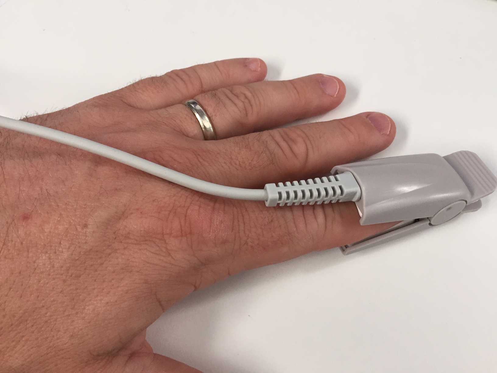
It features a red LED (660 nm) and an IR LED (900 nm) on the fingernail side and a photodiode for detecting transmitted light on the other side of the clip. The sensor probe has a male DE-9 connector. (You will see this referred to as a DB-9 in many places, but this is technically incorrect nomenclature.) The pins in a DE-9 connector are numbered as in the image below.
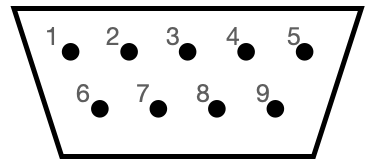
You should not directly used this geometry, though. Rather, you should plug the the connector on the sensor probe into the DE-9 female socket to terminal spring block adapter. This adapter allows you to plug jump wires into it, thereby connecting to the pins of the sensor probe. The ports on the block adapter are conveniently labeled with the pin numbers.
The pinout for the sensor probe is
Pin |
Purpose |
|---|---|
1 |
not used |
2 |
power/ground LEDs |
3 |
power/ground LEDs |
4 |
not used |
5 |
photodiode anode |
6 |
not used |
7 |
shield |
8 |
not used |
9 |
photodiode cathode |
The LEDs are connected to pins 2 and 3 as shown below.
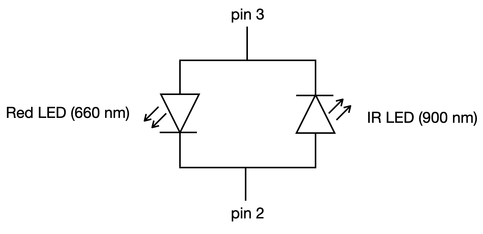
Note the polarity of the LEDs. Say you connected sensor probe pin 3 to 5 V (via a resistor of course) and pin 2 to ground. This would turn on the red LED. The IR LED would not turn on because it has the wrong polarity. Conversely, if you connected pin 2 to 5 V and pin 3 to ground, the IR LED would turn on, but the red LED would not turn on. Alternatively, you could leave pin 2 connected to ground and alternate between +5 V and –5 V supplied to pin 3 to switch between the red and IR LED being on, respectively.
IMPORTANT! Note that there are no resistors built-in to the sensor probe. You need to make sure you have a 220 Ω resistor connected to the voltage source you are using for the sensor probe LEDs! If you do not, you could destroy the sensor probe.
When connecting the photodiode, it is also important to connect it to a resistor. You can use the connection below.

You should also connect the shield to ground.
Because there is a single photodetector, you cannot simultaneously acquire a signal at the red and IR wavelengths. You therefore need to do the following.
Switch on the red LED.
Acquire a measurement.
Switch off the red LED.
Switch on the IR LED.
Acquire a measurement.
Switch off the IR LED.
Repeat.
You should also think about the following design considerations.
What sampling rate should you use to be able to resolve peaks and valleys in the cardiac cycle?
What kind of filtering is necessary?
Do you need to amplify the signals?
Do you need sample-and-hold circuits?
If you use those components, should you filter and/or amplify your signals before or after the sample-and-hold?